Antennas

RF Antenna Basics

                        Electromagnetic waves and antenna basics

Radio signals are a form of electromagnetic wave, and as they are the way in which radio signals travel, they have a major bearing on RF antennas themselves and RF antenna design. Electromagnetic waves are the same type of radiation as light, ultra-violet and infra red rays, differing from them in their wavelength and frequency. Electromagnetic waves have both electric and magnetic components that are inseparable. The planes of these fields are at right angles to one another and to the direction of motion of the wave. 

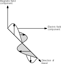
The electric field results from the voltage changes occurring in the RF antenna which is radiating the signal, and the magnetic changes result from the current flow. It is also found that the lines of force in the electric field run along the same axis as the RF antenna, but spreading out as they move away from it. This electric field is measured in terms of the change of potential over a given distance, e.g. volts per metre, and this is known as the field strength. Similarly when an RF antenna receives a signal the magnetic changes cause a current flow, and the electric field changes cause the voltage changes on the antenna.

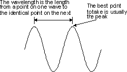
There are a number of properties of a wave. The first is its wavelength. This is the distance between a point on one wave to the identical point on the next. One of the most obvious points to choose is the peak as this can be easily identified although any point is acceptable.

Wavelength of an electromagnetic wave

 

The wavelength of an electromagnetic wave

The second property of the electromagnetic wave is its frequency. This is the number of times a particular point on the wave moves up and down in a given time (normally a second). The unit of frequency is the Hertz and it is equal to one cycle per second. This unit is named after the German scientist who discovered radio waves. The frequencies used in radio are usually very high. Accordingly the prefixes kilo, Mega, and Giga are often seen. 1 kHz is 1000 Hz, 1 MHz is a million Hertz, and 1 GHz is a thousand million Hertz i.e. 1000 MHz. Originally the unit of frequency was not given a name and cycles per second (c/s) were used. Some older books may show these units together with their prefixes: kc/s; Mc/s etc. for higher frequencies.

The third major property of the wave is its velocity. Radio waves travel at the same speed as light. For most practical purposes the speed is taken to be 300 000 000 metres per second although a more exact value is 299 792 500 metres per second.

 

Frequency to Wavelength Conversion

Although wavelength was used as a measure for signals, frequencies are used exclusively today. It is very easy to relate the frequency and wavelength as they are linked by the speed of light as shown:

lambda = c / f

where lambda = the wavelength in metres
f = frequency in Hertz
c = speed of radio waves (light) taken as 300 000 000 metres per second for all practical purposes.


 

Field measurements

It is also interesting to note that close to the RF antenna there is also an inductive field the same as that in a transformer. This is not part of the electromagnetic wave, but it can distort measurements close to the antenna. It can also mean that transmitting antennas are more likely to cause interference when they are close to other antennas or wiring that might have the signal induced into it. For receiving antennas they are more susceptible to interference if they are close to house wiring and the like. Fortunately this inductive field falls away fairly rapidly and it is barely detectable at distances beyond about two or three wavelengths from the RF antenna.

Antenna polarisation or polarization

- overview, summary, tutorial about RF antenna or aerial polarisation and the effect polarization has on RF antennas and radio communications.

Polarisation is an important factor for RF antennas and radio communications in general. Both RF antennas and electromagnetic waves are said to have a polarization. For the electromagnetic wave the polarization is effectively the plane in which the electric wave vibrates. This is important when looking at antennas because they are sensitive to polarisation, and generally only receive or transmit a signal with a particular polarization. For most antennas it is very easy to determine the polarization. It is simply in the same plane as the elements of the antenna. So a vertical antenna (i.e. one with vertical elements) will receive vertically polarised signals best and similarly a horizontal antenna will receive horizontally polarised signals.

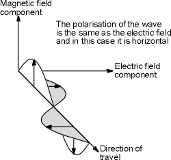
An electromagnetic wave

It is important to match the polarization of the RF antenna to that of the incoming signal. In this way the maximum signal is obtained. If the RF antenna polarization does not match that of the signal there is a corresponding decrease in the level of the signal. It is reduced by a factor of cosine of the angle between the polarisation of the RF antenna and the signal.

Accordingly the polarisation of the antennas located in free space is very important, and obviously they should be in exactly the same plane to provide the optimum signal. If they were at right angles to one another (i.e. cross-polarised) then in theory no signal would be received.

For terrestrial radio communications applications it is found that once a signal has been transmitted then its polarisation will remain broadly the same. However reflections from objects in the path can change the polarisation. As the received signal is the sum of the direct signal plus a number of reflected signals the overall polarisation of the signal can change slightly although it remains broadly the same.

 

Polarisation catagories

Vertical and horizontal are the simplest forms of antenna polarization and they both fall into a category known as linear polarisation. However it is also possible to use circular polarisation. This has a number of benefits for areas such as satellite applications where it helps overcome the effects of propagation anomalies, ground reflections and the effects of the spin that occur on many satellites. Circular polarisation is a little more difficult to visualise than linear polarisation. However it can be imagined by visualising a signal propagating from an RF antenna that is rotating. The tip of the electric field vector will then be seen to trace out a helix or corkscrew as it travels away from the antenna. Circular polarisation can be seen to be either right or left handed dependent upon the direction of rotation as seen from the transmitter.

Another form of polarisation is known as elliptical polarisation. It occurs when there is a mix of linear and circular polarisation. This can be visualised as before by the tip of the electric field vector tracing out an elliptically shaped corkscrew.

However it is possible for linearly polarised antennas to receive circularly polarised signals and vice versa. The strength will be equal whether the linearly polarised antenna is mounted vertically, horizontally or in any other plane but directed towards the arriving signal. There will be some degradation because the signal level will be 3 dB less than if a circularly polarised antenna of the same sense was used. The same situation exists when a circularly polarised antenna receives a linearly polarised signal.

 

Applications of antenna polarization

Different types of polarisation are used in different applications to enable their advantages to be used. Linear polarization is by far the most widely used for most radio communications applications. Vertical polarisation is often used for mobile radio communications. This is because many vertically polarized antenna designs have an omni-directional radiation pattern and it means that the antennas do not have to be re-orientated as positions as always happens for mobile radio communications as the vehicle moves. For other radio communications applications the polarisation is often determined by the RF antenna considerations. Some large multi-element antenna arrays can be mounted in a horizontal plane more easily than in the vertical plane. This is because the RF antenna elements are at right angles to the vertical tower of pole on which they are mounted and therefore by using an antenna with horizontal elements there is less physical and electrical interference between the two. This determines the standard polarisation in many cases.

In some applications there are performance differences between horizontal and vertical polarization. For example medium wave broadcast stations generally use vertical polarisation because ground wave propagation over the earth is considerably better using vertical polarization, whereas horizontal polarization shows a marginal improvement for long distance communications using the ionosphere. Circular polarisation is sometimes used for satellite radio communications as there are some advantages in terms of propagation and in overcoming the fading caused if the satellite is changing its orientation.

Antenna feed impedance

When a signal source is applied to an RF antenna at its feed point, it is found that it presents a load impedance to the source. This is known as the antenna "feed impedance" and it is a complex impedance made up from resistance, capacitance and inductance. In order to ensure the optimum efficiency for any RF antenna design it is necessary to maximise the transfer of energy by matching the feed impedance of the RF antenna design to the load. This requires some understanding of the operation of antenna design in this respect.

The feed impedance of the antenna results from a number of factors including the size and shape of the RF antenna, the frequency of operation and its environment. The impedance seen is normally complex, i.e. consisting of resistive elements as well as reactive ones.

Antenna feed impedance resistive elements

The resistive elements are made up from two constituents. These add together to form the sum of the total resistive elements.

• Loss resistance:   The loss resistance arises from the actual resistance of the elements in the aRF ntenna, and power dissipated in this manner is lost as heat. Although it may appear that the "DC" resistance is low, at higher frequencies the skin effect is in evidence and only the surface areas of the conductor are used. As a result the effective resistance is higher than would be measured at DC. It is proportional to the circumference of the conductor and to the square root of the frequency.
  
  The resistance can become particularly significant in high current sections of an RF antenna where the effective resistance is low. Accordingly to reduce the effect of the loss resistance it is necessary to ensure the use of very low resistance conductors.
  
  
• Radiation resistance:   The other resistive element of the impedance is the "radiation resistance". This can be thought of as virtual resistor. It arises from the fact that power is "dissipated" when it is radiated from the Rf antenna. The aim is to "dissipate" as much power in this way as possible. The actual value for the radiation resistance varies from one type of antenna to another, and from one design to another. It is dependent upon a variety of factors. However a typical half wave dipole operating in free space has a radiation resistance of around 73 Ohms.
  

Reactive elements

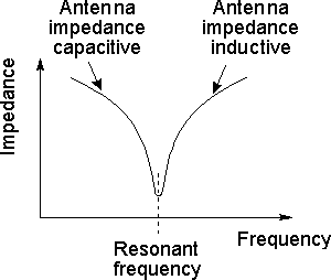
There are also reactive elements to the feed impedance. These arise from the fact that the antenna elements act as tuned circuits that possess inductance and capacitance. At resonance where most antennas are operated the inductance and capacitance cancel one another out to leave only the resistance of the combined radiation resistance and loss resistance. However either side of resonance the feed impedance quickly becomes either inductive (if operated below the resonant frequency) or capacitive (if operated above the resonant frequency).

Efficiency

It is naturally important to ensure that the proportion of the power dissipated in the loss resistance is as low as possible, leaving the highest proportion to be dissipated in the radiation resistance as a radiated signal. The proportion of the power dissipated in the radiation resistance divided by the power applied to the antenna is the efficiency.

A variety of means can be employed to ensure that the efficiency remains as high as possible. These include the use of optimum materials for the conductors to ensure low values of resistance, large circumference conductors to ensure large surface area to overcome the skin effect, and not using designs where very high currents and low feed impedance values are present. Other constraints may require that not all these requirements can be met, but by using engineering judgement it is normally possible to obtain a suitable compromise.

Summary

It can be seen that the antenna feed impedance is particularly important when considering any RF antenna design. However by maximising the energy transfer by matching the feeder to the antenna feed impedance the antenna design can be optimised and the best performance obtained.

Antenna resonance and bandwidth

Two major factors associated with radio antenna design are the antenna resonant point or centre operating frequency and the antenna bandwidth or the frequency range over which the antenna design can operate. These two factors are naturally very important features of any antenna design and as such they are mentioned in specifications for particular RF ntennas. Whether the RF antenna is used for broadcasting, WLAN, cellular telecommunications, PMR or any other application, the performance of the RF antenna is paramount, and the antenna resonant frequency and the antenna bandwidth are of great importance.

Antenna resonance

An RF antenna is a form of tuned circuit consisting of inductance and capacitance, and as a result it has a resonant frequency. This is the frequency where the capacitive and inductive reactances cancel each other out. At this point the RF antenna appears purely resistive, the resistance being a combination of the loss resistance and the radiation resistance.

Impedance of an RF antenna with frequency

The capacitance and inductance of an RF antenna are determined by its physical properties and the environment where it is located. The major feature of the RF antenna design is its dimensions. It is found that the larger the antenna or more strictly the antenna elements, the lower the resonant frequency. For example antennas for UHF terrestrial television have relatively small elements, while those for VHF broadcast sound FM have larger elements indicating a lower frequency. Antennas for short wave applications are larger still.

Antenna bandwidth

Most RF antenna designs are operated around the resonant point. This means that there is only a limited bandwidth over which an RF antenna design can operate efficiently. Outside this the levels of reactance rise to levels that may be too high for satisfactory operation. Other characteristics of the antenna may also be impaired away from the centre operating frequency.

The antenna bandwidth is particularly important where radio transmitters are concerned as damage may ccur to the transmitter if the antenna is operated outside its operating range and the radio transmitter is not adequately protected. In addition to this the signal radiated by the RF antenna may be less for a number of reasons.

For receiving purposes the performance of the antenna is less critical in some respects. It can be operated outside its normal bandwidth without any fear of damage to the set. Even a random length of wire will pick up signals, and it may be possible to receive several distant stations. However for the best reception it is necessary to ensure that the performance of the RF antenna design is optimum.

Impedance bandwidth

One major feature of an RF antenna that does change with frequency is its impedance. This in turn can cause the amount of reflected power to increase. If the antenna is used for transmitting it may be that beyond a given level of reflected power damage may be caused to either the transmitter or the feeder, and this is quite likely to be a factor which limits the operating bandwidth of an antenna. Today most transmitters have some form of SWR protection circuit that prevents damage by reducing the output power to an acceptable level as the levels of reflected power increase. This in turn means that the efficiency of the station is reduced outside a given bandwidth. As far as receiving is concerned the impedance changes of the antenna are not as critical as they will mean that the signal transfer from the antenna itself to the feeder is reduced and in turn the efficiency will fall. For amateur operation the frequencies below which a maximum SWR figure of 1.5:1 is produced is often taken as the acceptable bandwidth.

In order to increase the bandwidth of an antenna there are a number of measures that can be taken. One is the use of thicker conductors. Another is the actual type of antenna used. For example a folded dipole which is described fully in Chapter 3 has a wider bandwidth than a non-folded one. In fact looking at a standard television antenna it is possible to see both of these features included.

Radiation pattern

Another feature of an antenna that changes with frequency is its radiation pattern. In the case of a beam it is particularly noticeable. In particular the front to back ratio will fall off rapidly outside a given bandwidth, and so will the gain. In an antenna such as a Yagi this is caused by a reduction in the currents in the parasitic elements as the frequency of operation is moved away from resonance. For beam antennas such as the Yagi the radiation pattern bandwidth is defined as the frequency range over which the gain of the main lobe is within 1 dB of its maximum.

For many beam antennas, especially high gain ones it will be found that the impedance bandwidth is wider than the radiation pattern bandwidth, although the two parameters are inter-related in many respects.

Antenna directivity and gain

 

RF antennas or aerials do not radiate equally in all directions. It is found that any realisable RF antenna design will radiate more in some directions than others. The actual pattern is dependent upon the type of antenna design, its size, the environment and a variety of other factors. This directional pattern can be used to ensure that the power radiated is focussed in the desired directions.

It is normal to refer to the directional patterns and gain in terms of the transmitted signal. It is often easier to visualise the RF antenna is terms of its radiated power, however the antenna performs in an exactly equivalent manner for reception, having identical figures and specifications.

In order to visualise the way in which an antenna radiates a diagram known as a polar diagram is used. This is normally a two dimensional plot around an antenna showing the intensity of the radiation at each point for a particular plane. Normally the scale that is used is logarithmic so that the differences can be conveniently seen on the plot. Although the radiation pattern of the antenna varies in three dimensions, it is normal to make a plot in a particular plane, normally either horizontal or vertical as these are the two that are most used, and it simplifies the measurements and presentation. An example for a simple dipole antenna is shown below.

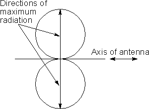
Polar diagram of a half wave dipole in free space

Antenna designs are often categorised by the type of polar diagram they exhibit. For example an omni-directional antenna design is one which radiates equally (or approximately equally) in all directions in the plane of interest. An antenna design that radiates equally in all directions in all planes is called an isotropic antenna. As already mentioned it is not possible to produce one of these in reality, but it is useful as a theoretical reference for some measurements. Other RF antennas exhibit highly directional patterns and these may be utilised in a number of applications. The Yagi antenna is an example of a directive antenna and possibly it is most widely used for television reception.

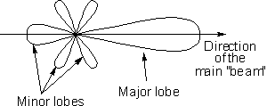
Polar diagram for a yagi antenna

RF antenna beamwidth

There are a number of key features that can be seen from this polar diagram. The first is that there is a main beam or lobe and a number of minor lobes. It is often useful to define the beam-width of an RF antenna. This is taken to be angle between the two points where the power falls to half its maximum level, and as a result it is sometimes called the half power beam-width.

Antenna gain

An RF antenna radiates a given amount of power. This is the power dissipated in the radiation resistance of the RF antenna. An isotropic radiator will distribute this equally in all directions. For an antenna with a directional pattern, less power will be radiated in some directions and more in others. The fact that more power is radiated in given directions implies that it can be considered to have a gain.

The gain can be defined as a ratio of the signal transmitted in the "maximum" direction to that of a standard or reference antenna. This may sometimes be called the "forward gain". The figure that is obtained is then normally expressed in decibels (dB). In theory the standard antenna could be almost anything but two types are generally used. The most common type is a simple dipole as it is easily available and it is the basis of many other types of antenna. In this case the gain is often expressed as dBd i.e. gain expressed in decibels over a dipole. However a dipole does not radiated equally in all directions in all planes and so an isotropic source is sometimes used. In this case the gain may be specified in dBi i.e. gain in decibels over an isotropic source. The main drawback with using an isotropic source (antenna dBi) as a reference is that it is not possible to realise them in practice and so that figures using it can only be theoretical. However it is possible to relate the two gains as a dipole has a gain of 2.1 dB over an isotropic source i.e. 2.1 dBi. In other words, figures expressed as gain over an isotropic source will be 2.1 dB higher than those relative to a dipole. When choosing an antenna and looking at the gain specifications, be sure to check whether the gain is relative to a dipole or an isotropic source, i.e. the antenna dBi figure of the antenna dBd figure.

Apart from the forward gain of an antenna another parameter which is important is the front to back ratio. This is expressed in decibels and as the name implies it is the ratio of the maximum signal in the forward direction to the signal in the opposite direction. This figure is normally expressed in decibels. It is found that the design of an antenna can be adjusted to give either maximum forward gain of the optimum front to back ratio as the two do not normally coincide exactly. For most VHF and UHF operation the design is normally optimised for the optimum forward gain as this gives the maximum radiated signal in the required direction.

RF antenna gain / beamwidth balance

It may appear that maximising the gain of an antenna will optimise its performance in a system. This may not always be the case. By the very nature of gain and beamwidth, increasing the gain will result in a reduction in the beamwidth. This will make setting the direction of the antenna more critical. This may be quite acceptable in many applications, but not in others. This balance should be considered when designing and setting up a radio link.RF coax cable connectors

A wide variety of RF connectors are available for making connections to coaxial cable. These connectors including BNC, C-type, N-type, UHF (Amphenol) connector, SMA, SMB, SMC and many more are able to be used in a variety of applications.

RF Coax Cable Connectors

Coax cable connectors, often called RF connectors are in widespread use. Wherever radio frequency or RF connections need to be made there is the possibility of using coaxial connectors. Where signals reach frequencies above a few million Hertz, these coaxial connectors need to be used. The need for their use arises because it is necessary to transfer radio frequency, RF, energy from one place to another using a transmission line. The most convenient, and hence the most commonly used form of transmission line is coaxial cable which consists of two concentric conductors, an inner conductor and an outer conductor, often called the screen. Between these two conductors there is an insulating dielectric.

Coaxial cable has a number of properties, one of which is the characteristic impedance. In order that the maximum power transfer takes place from the source to the load, the characteristic impedances of both should match. Thus the characteristic impedance of a feeder is of great importance. Any mismatch will result in power being reflected back towards the source.

It is also important that RF coaxial cable connectors have a characteristic impedance that matches that of the cable. If not, a discontinuity is introduced and losses may result.

There is a variety of connectors that are used for RF applications. Impedance, frequency range, power handling, physical size and a number of other parameters including cost will determine the best type for a given applications.

UHF connector

The UHF connector, also sometimes known as the Amphenol coaxial connector was designed in the 1930s by a designer in the Amphenol company for use in the radio industry. The plug may be referred to as a PL259 coaxial connector, and the socket as an SO239 connector. These are their original military part numbers

These coaxial connectors have a threaded coupling, and this prevents them from being removed accidentally. It also enables them to be tightened sufficiently to enable a good low resistance connection to be made between the two halves.

The drawback of the UHF or Amphenol connector is that it has a non-constant impedance. This limits their use to frequencies of up to 300 MHz, but despite this these UHF connectors provide a low cost connector suitable for many applications, provided that the frequencies do not rise. Also very low cost versions are available for applications such as CB operation, and these are not suitable for operation much above 30 MHz. In view of their non-constant impedance, these connectors are now rarely used for many professional applications, being generally limited to CB, amateur radio and some video and public address systems.

N-type connector

The N-type connector is a high performance RF coaxial connector used in many RF applications. This coax connector was designed by Paul Neill of Bell Laboratories, and it gained its name from the first letter of his surname.

This RF connector has a threaded coupling interface to ensure that it mates correctly. It is available in either 50 ohm or 75 ohm versions. These two versions have subtle mechanical differences that do not allow the two types to mate. The connector is able to withstand relatively high powers when compared to the BNC or TNC connectors. The standard versions are specified for operation up to 11 GHz, although precision versions are available for operation to 18GHz.

The N-type coaxial connector is used for many radio frequency applications including broadcast and communications equipment where its power handling capability enables it to be used for medium power transmitters, however it is also used for many receivers and general RF applications.

BNC connector

The BNC coax connector is widely used in professional circles being used on most oscilloscopes and many other laboratory instruments. The BNC connector is also widely used when RF connections need to be made. The BNC connector has a bayonet fixing to prevent accidental disconnection while being easy to disconnect when necessary. This RF connector was developed in the late 1940s and it gains its name from a combination of the fact that it has a bayonet fixing and from the names of the designers, the letters BNC standing for Bayonet Neill Concelman. In fact the BNC connector is essentially a miniature version of the C connector which was a bayonet version of the N-type connector.

Electrically the BNC coax cable connector is designed to present a constant impedance and it is most common in its 50 ohm version, although 75 ohm ones can be obtained. It is recommended for operation at frequencies up to 4 GHz and it can be used up to 10 GHz provided the special top quality versions specified to that frequency are used.

TNC connector

The TNC connector is very similar to the BNC connector. The main difference is that it has a screw fitting instead of the bayonet one. The TNC connector was developed originally to overcome problems during vibration. As the bayonet fixing moved slightly there were small changes to the resistance of the connections and this introduced noise. To solve the problem a screw fixing was used and the TNC coax cable connector gains its name from the words Threaded Neill Concelman.

Like the BNC connector, the TNC connector has a constant impedance, and in view of the threaded connection, its frequency limit can be extended. Most TNC connectors are specified to 11 GHz, and some may be able to operate to 18 GHz.

SMA connector

This sub-miniature RF coaxial cable connector takes its name from the words Sub-Miniature A connector. It finds many applications for providing connectivity for RF assemblies within equipments. It is often used for providing RF connectivity between boards, and many microwave components including filters, attenuators, mixers and oscillators, use SMA connectors.

The connectors have a threaded outer coupling interface that has a hexagonal shape, allowing it to be tightened with a spanner. Special torque spanners are available to enable them to be tightened to the correct tightness, allowing a good connection to be made without over-tightening them.

The SMA connector was originally designed in the 1960s for use with 141 semi-rigid coax cable. Here the centre of the coax forms the centre pin for the connection, removing the necessity for a transition between the coax centre conductor and a special connector centre pin. However its use extended to other flexible cables, and connectors with centre pins were introduced.

SMA connectors are regularly used for frequencies well into the microwave region, and some versions may be used at frequencies up to 26.5 GHz. For flexible cables, the frequency limit is normally determined by the cable and not the connector.

SMB connector

The SMB connector derives its name as it is termed a Sub-Miniature B connector. It was developed as a result of the need for a connector that was able to connect and disconnect swiftly. It does not require nuts to be tightened when two connectors are mated. Instead the connectors are brought together and they snap fit together. Additionally the connector utilizes an inner contact and overlapping dielectric insulator structures to ensure good connectivity and a constant impedance.

SMB coaxial connectors perform well under moderate vibration only and the 50 ohm versions are often specified to 4 GHz. 75 ohm versions of the SMB coaxial connector are also available, but there are often not specified up to the same frequencies, often only about 2GHz.

SMB coaxial connectors are not as widely used as their SMA counterparts. They are used for inter board or assembly connections within equipment, although they are not widely used for purchased microwave assemblies in view of their inferior performance.

SMC connector

A third SM type connector is not surprisingly the Sub Miniature C or SMC coaxial cable connector. It is similar to the SMB connector, but it uses a threaded coupling interface rather than the snap-on connection. This provides a far superior interface for the connection and as a result, SMC coaxial cable connectors are normally specified to operate at frequencies up to 10 GHz.

SMC coaxial cable connectors provide a good combination of small size and performance. They may also be used in environments where vibration is anticipated. In view of their performance they find applications in microwave equipment, although they are not normally used for military applications where SMA connectors tend to be preferred.

MCX connector

A number of mico-miniatiure RF connectors have been developed by a variety of manufacturers to meet the growing demand for cost effective, high quality smaller connectors. These are finding high levels of use, for example in the cellular phone industry, where size, cost and performance are all important. In fact the MCX is about 30% smaller in both size and weight than an SMB connector to which it has many similarities.

One connector that falls into this category is the MCX (MicroCoaX) coax connector. This was developed in the 1980s by Huber and Suhner of which MCX is a trade name. The MCX connector has many similarities with the construction of the SMB connector using a quick snap-on interface, and utilising an inner contact and an overlapping dielectric insulator structure.

The MCX connector is normally specified for operation up to 6 GHz, and it finds applications in a variety of arenas including equipment for cellular telecommunications, data telemetry, Global positioning (GPS) and other applications where size and weight are important and frequencies are generally below 5 GHz.

MMCX connector

Another connector which is being widely used is the MMCX connector. Being some 45% smaller than an SMB connector, the MMCX is ideal where a low profile outline is a key element. It is therefore ideal for applications where board height is limited, including applications where boards may be stacked. As such it is being widely used in many cellular telecommunications applications.

The connector provides a snap fitting and also utilises a slot-less design to minimise leakage.

Overview

There is a great variety of RF coaxial cable connectors in use today. The list above describes some of the more popular types of RF connector, but there are nevertheless more varieties available. When choosing a coaxial cable connector, the requirements should be carefully matched to the available options to see which RF connector will provide the best choice. In this way the best compromise between size, weight, performance and cost can be achieved.

BNC connector

The BNC coax connector is a form of rf connector that is one of the most widely used coaxial connectors. The BNC connector is intended as an RF connector that can be used in a wide number of applications from any form of RF equipment including radio communications equipment to test equipment including everything from oscilloscopes to audio generators, and power meters to function generators. In fact BNC connectors are used in applications where coaxial or screened cable is required.

The BNC connector has many attributes. One is that it has a bayonet fixing. This is particularly useful because it prevents accidental disconnection if the cable is pulled slightly or repeatedly moved. Another advantage is that it is what is termed a constant impedance connector. This is particularly important for RF applications and means that the connector presents the same impedance throughout its length.

BNC development

The BNC connector was developed in the late 1940s and it gains its name from a combination of the fact that it has a bayonet fixing and from the names of the designers, the letters BNC standing for Bayonet Neill Concelman. In fact the BNC connector is essentially a miniature version of the C connector which was a bayonet version of the N-type connector.

It was developed as a result of the need to provide a high quality, robust connector that would be capable of being used in a wide variety of applications. Additionally it needed to be smaller than either the N-type or C-type connectors which were much larger

BNC connector specifications

The specifications of the BNC connector naturally vary from one manufacturer to another and it is always best to ensure that the particular component being purchased is suitable for the intended application. However there are a number of guidelines that can be used. The connector comes in two basic types:

• 50 ohm
  
  
• 75 ohm
  
  

Of the two versions of the BNC connector, the 50 ohm version is more widely used. Often the BNC connector is specified for operation at frequencies up to 4 GHz and it can be used up to 10 GHz provided the special top quality versions specified to that frequency are used. However it is wise to fully check the specification.

BNC connector formats

BNC connectors come in a variety of formats. Not only are there plugs and sockets but there are also adapters and also other items such as attenuators.

BNC plugs are designed not only for the required impedance, but also to accept a particular coax cable format. In this way all the internal piece parts are compatible with the coaxial cable used. It is therefore necessary to specify the BNC plug for use the cable to be used. Although there is some latitude, it is naturally best to select the correct cable format.

In addition to this there are straight and right angled variants. Of these the straight connectors are the most widely used, although right angled connectors where the cable leaves the plug at right angles to the centre of the connector centre line are also available. These are ideal in many applications where the cables need to leave the connector in this manner to ensure cables are in a tidy fashion, or where space is at a premium. Unfortunately right-angled connectors have a marginally higher level of loss than their straight through counterparts. This may not be significant for most applications, but at frequencies near the operational limit of the connector there may be a small difference.

The sockets or female BNC connectors also come in a number of flavours. The very basic BNC connector consists of a panel mounting assembly with a single connection for the coax centre. The earthing is then accomplished via the panel to which the connector is bolted using a single nut. Large washers can be used to provide an earth connection directly to the connector. Some of these connectors may also use four nuts and bolts to fix them to the panel. These arrangements are only suitable for low frequency applications, and not for RF. Where impedance matching and full screening is required. Bulkhead mounting connectors where coaxial cable entry is provided are available for this. Again these are available for a variety of cable dimensions and the correct type should be used.

There are two main variants of the BNC connector assembly method:

• Compression gland type
  
  
• Crimp type
  

The compression gland type has the centre pin of the connector which is usually a solder pin and the braid and sheath of the cable are held by an expanding compression gland fixed by a nut at the rear of the connector. This type of connector by its nature can cope with a (limited) range of cable sizes and requires no specialised tooling to assemble. This makes it ideal for small quantity production, either for one off cables for laboratory use of for limited production runs.

The crimp connector has the centre pin which is normally crimped to the centre conductor. This crimped pin is then pushed into position through an inner ferrule which separates the inner insulation sheath and the braid of the cable. An outer ferrule is then crimped over the braid and outer insulation which fixes the cable to the connector. Greater accuracy is required for the crimp style connectors and therefore the correct connector variant must be chosen for the cable being used. This may result in a crimp style connector not being practicable for some cable types. In addition to this the assembly requires the use of the correct crimping tools to ensure that the connector is correctly crimped. While these connectors are always preferred for large production runs because they are much faster to assemble, it is not possible for them to be reworked for obvious reasons.

For both styles of BNC connector it is essential that the exact amount of insulation is stripped from each section to ensure accurate assembly and the required RF performance.

Finally a variety of BNC adapters and other ancillary items are available. One popular BNC adapter is the straight through adapter, allowing two cables with male connectors fitted to be connected end to end. Other "T" adapters are also available. These have a male plug at the bottom of the "T" and two female connections at either end of the horizontal of the "T". These are ideal for use with oscilloscopes where a through connection needs to be measured, and the "T" BNC adapter enables the required connections to be made.

In addition to this a variety of inter-series adapters are available to enable transitions to be made between different connector types.

TNC connector

The TNC connector is very similar to the BNC connector although it is not nearly as widely used. The main difference between then is that the TNC connector has a screw fitting instead of the bayonet. The screw fitting means that the RF connection of the TNC connector is generally more robust and accordingly it can operate more reliably at higher frequencies.

Development

The TNC connector was developed originally to overcome problems during vibration. As the bayonet fixing moved slightly there were small changes to the resistance of the connections and this introduced noise. To solve the problem a screw fixing was used and the TNC coax cable connector gains its name from the words Threaded Neill Concelman.

TNC connector performance

Like the BNC connector, the TNC connector has a constant impedance, and in view of the threaded connection, its frequency limit can be extended. Most TNC connectors are specified to 11 GHz, and some are able to operate to 18 GHz.

TNC connector formats

TNC connectors come in a variety of formats. Not only are there plugs and sockets but there are also adapters and also other items such as attenuators.

TNC plugs are designed not only for the required impedance, but also to accept a particular coax cable format. In this way all the internal piece parts are compatible with the coaxial cable used. It is therefore necessary to specify the TNC plug for use the cable to be used. Although there is some latitude, it is naturally best to select the correct cable format.

In addition to this there are straight and right angled variants. Of these the straight connectors are the most widely used, although right angled connectors where the cable leaves the plug at right angles to the centre of the connector centre line are also available. These are ideal in many applications where the cables need to leave the connector in this manner to ensure cables are in a tidy fashion, or where space is at a premium. Unfortunately right-angled connectors have a marginally higher level of loss than their straight through counterparts. This may not be significant for most applications, but at frequencies near the operational limit of the connector there may be a small difference.

The sockets or female BNC connectors also come in a number of flavours. The very basic BNC connector consists of a panel mounting assembly with a single connection for the coax centre. The earthing is then accomplished via the panel to which the connector is bolted using a single nut. Large washers can be used to provide an earth connection directly to the connector. Some of these connectors may also use four nuts and bolts to fix them to the panel. These arrangements are only suitable for low frequency applications, and not for RF. Where impedance matching and full screening is required. Bulkhead mounting connectors where coaxial cable entry is provided are available for this. Again these are available for a variety of cable dimensions and the correct type should be used.

There are two main variants of the TNC connector assembly method:

• Compression gland type
  
  
• Crimp type
  

The compression gland type has the centre pin of the connector which is usually a solder pin and the braid and sheath of the cable are held by an expanding compression gland fixed by a nut at the rear of the connector. This type of connector by its nature can cope with a (limited) range of cable sizes and requires no specialised tooling to assemble. This makes it ideal for small quantity production, either for one off cables for laboratory use of for limited production runs.

The crimp TNC connector has the centre pin which is normally crimped to the centre conductor. This crimped pin is then pushed into position through an inner ferrule which separates the inner insulation sheath and the braid of the cable. An outer ferrule is then crimped over the braid and outer insulation which fixes the cable to the connector. Greater accuracy is required for the crimp style connectors and therefore the correct connector variant must be chosen for the cable being used. This may result in a crimp style connector not being practicable for some cable types. In addition to this the assembly requires the use of the correct crimping tools to ensure that the connector is correctly crimped. While these connectors are usually preferred for large production runs because they are faster to assemble, it is not possible for them to be reworked for obvious reasons.

For both styles of TNC connector it is essential that the exact amount of insulation is stripped from each section to ensure accurate and successful assembly.

The sockets or female TNC connectors also come in a number of flavours. In view of the fact that TNC connectors are normally used for RF applications, bulkhead mounting connectors where coaxial cable entry is provided are normally used. Again these are available for a variety of cable dimensions and the correct type should be used.